How To Add Another Set Of Data In Excel Graph

Lesson 22: Charts

/en/excel2013/tables/content/

Introduction

Information technology can ofttimes be hard to interpret Excel workbooks that contain a lot of data. Charts allow yous to illustrate your workbook data graphically, which makes information technology piece of cake to visualize comparisons and trends.

Optional: Download our practice workbook.

Understanding charts

Excel has several unlike types of charts, allowing you lot to choose the 1 that best fits your data. In order to apply charts effectively, yous'll need to understand how different charts are used.

Click the arrows in the slideshow below to larn more nearly the types of charts in Excel.

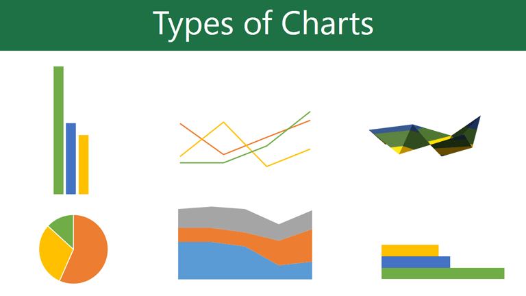
Excel has a variety of chart types, each with its ain advantages. Click the arrows to encounter some of the different types of charts available in Excel.
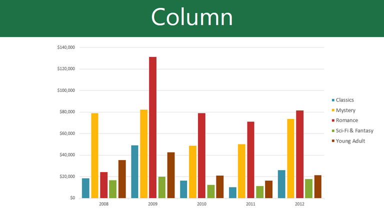
Column charts use vertical confined to represent data. They can work with many different types of data, simply they're about frequently used for comparing data.
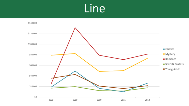
Line charts are ideal for showing trends. The information points are connected with lines, making it easy to see whether values are increasing or decreasing over time.
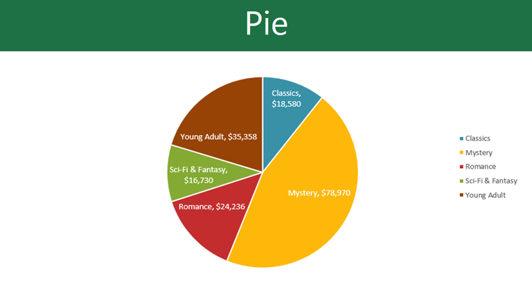
Pie charts make it like shooting fish in a barrel to compare proportions. Each value is shown as a slice of the pie, so information technology'due south easy to see which values make upwardly the per centum of a whole.
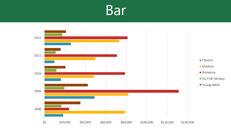
Bar charts piece of work just like column charts, only they use horizontal bars instead of vertical bars.
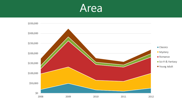
Expanse charts are similar to line charts, except the areas under the lines are filled in.
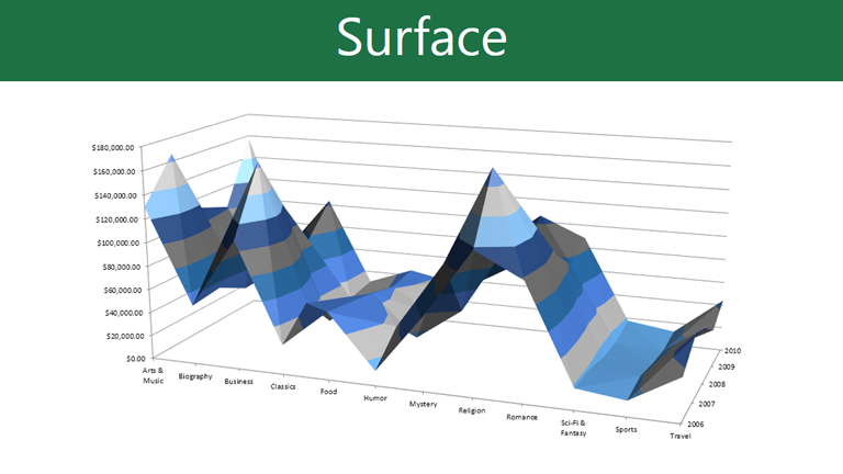
Surface charts allow you to display data across a 3D mural. They work best with large data sets, allowing you to run across a variety of information at the aforementioned fourth dimension.

In addition to chart types, you'll need to sympathise how to read a chart. Charts contain several different elements, or parts, that can aid yous interpret the data.

Click the buttons in the interactive beneath to learn about the different parts of a chart.

labeled graphic

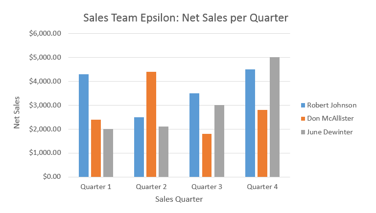
Legend

The legend identifies which data series each color on the chart represents.

In this case, the legend identifies the different salespeople in the nautical chart.

Chart Title

The championship should clearly describe what the nautical chart is illustrating.

Vertical Axis

The vertical centrality (as well known as the y axis ) is the vertical part of the chart.

Here, the vertical axis measures the value of the columns, and then it is too called the value axis. In this example, the measured value is each salesperson's net sales.

Horizontal Axis

The horizontal axis (also known every bit the x axis ) is the horizontal part of the nautical chart.

Here, the horizontal axis identifies the categories in the chart. In this instance, each sales quarter is placed in its ain group.

Data Series

The data serial consists of the related data points in a chart.

In this example, the blueish columns represent net sales by Robert Johnson. We know his data is blue considering of the legend on the right.

Reading the data series, we can see that Robert was the meridian salesperson in quarters i and 3, while he was the 2nd highest in quarters 2 and four.

To insert a nautical chart:

Select the cells y'all desire to chart, including the column titles and row labels. These cells will exist the source data for the chart. In our instance, we'll select cells A1:F6.
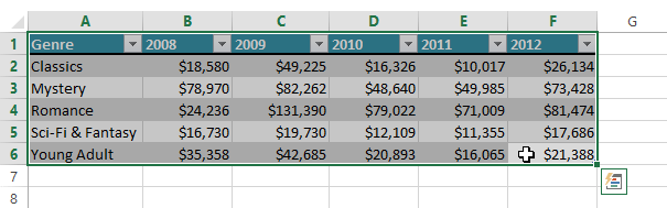Selecting cells A1:F6
From the Insert tab, click the desired Chart command. In our example, nosotros'll select Cavalcade.
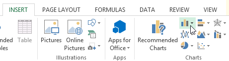Clicking the Column chart command
Choose the desired chart type from the driblet-down menu.
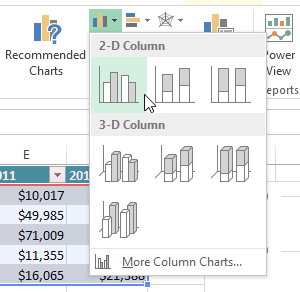Choosing a chart type
The selected nautical chart will be inserted in the worksheet.
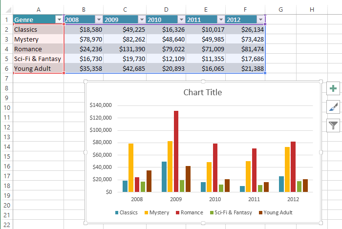The inserted chart

If you're non sure which type of nautical chart to utilize, the Recommended Charts command volition suggest several different charts based on the source data.

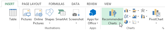Screenshot of Excel 2013 Clicking the Recommended Charts control

Nautical chart layout and style

After inserting a chart, in that location are several things you may want to change about the fashion your information is displayed. It'due south piece of cake to edit a chart'due south layout and mode from the Design tab.

Excel allows yous to add nautical chart elements—such as chart titles, legends, and data labels—to make your chart easier to read. To add a chart element, click the Add together Chart Element command on the Design tab, then choose the desired chemical element from the drop-down menu.

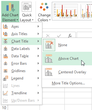
Adding a chart championship
To edit a chart chemical element, like a chart title, simply double-click the placeholder and begin typing.
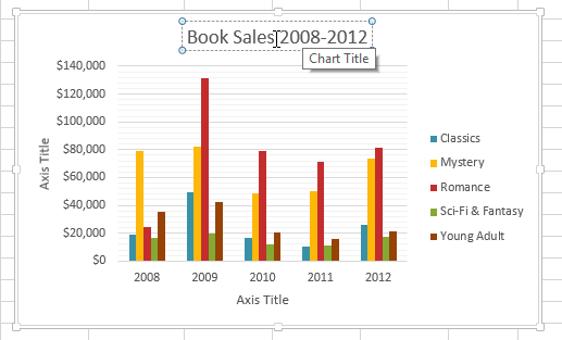Editing the chart title placeholder text
If yous don't want to add chart elements individually, you tin can utilize one of Excel'southward predefined layouts. Merely click the Quick Layout command, then cull the desired layout from the drop-downwardly carte du jour.
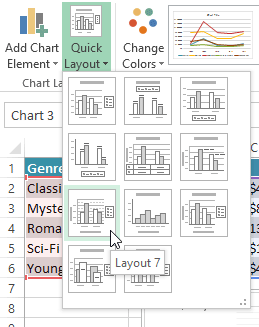Choosing a nautical chart layout
Excel too includes several different chart styles, which allow you to quickly modify the look and experience of your nautical chart. To modify the nautical chart style, select the desired style from the Chart styles group.
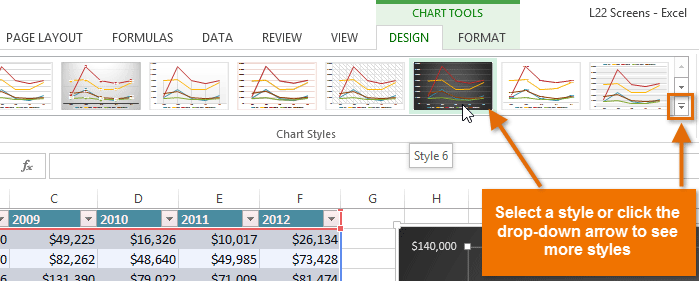Choosing a new chart style

You can besides apply the chart formatting shortcut buttons to quickly add together nautical chart elements, change the chart style, and filter the chart information.

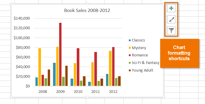Screenshot of Excel 2013 Nautical chart formatting shortcuts

Other chart options

There are many other ways to customize and organize your charts. For example, Excel allows y'all to rearrange a chart's information, change the chart type, and even motion the chart to a unlike location in the workbook.

To switch row and column information:

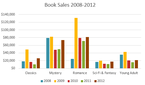
Sometimes you may want to change the manner charts group your information. For instance, in the chart below, the Book Sales information are grouped by year, with columns for each genre. Yet, we could switch the rows and columns so the chart will grouping the data past genre, with columns for each twelvemonth. In both cases, the chart contains the same information—it's but organized differently.

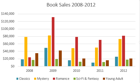Screenshot of Excel 2013 The data grouped by year, with columns for each genre

Select the chart yous want to change.
From the Design tab, select the Switch Row/Cavalcade command.

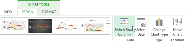Clicking the Switch Rows/Columns command
The rows and columns will be switched. In our example, the data is now grouped by genre, with columns for each year.
The switched row and column data

To change the chart blazon:

If you notice that your information isn't well suited to a certain chart, it's easy to switch to a new chart type. In our example, we'll change our chart from a Column nautical chart to a Line chart.

From the Pattern tab, click the Alter Chart Type command.
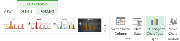Clicking the Change Chart Type control
The Change Nautical chart Type dialog box will appear. Select a new chart type and layout, then click OK. In our instance, we'll choose a Line chart.
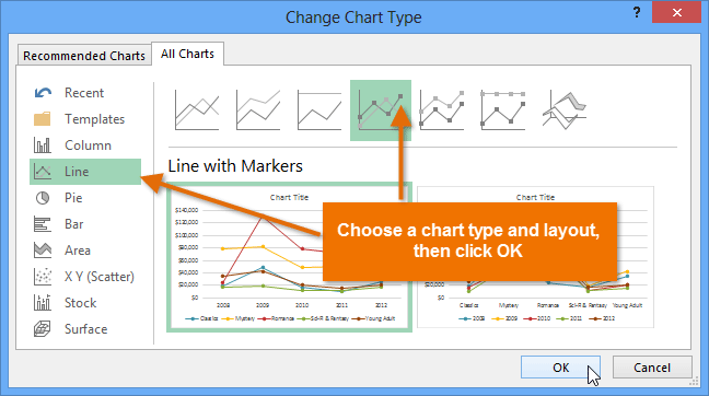Choosing a new chart type
The selected nautical chart type will appear. In our instance, the line chart makes it easier to meet trends in the sales data over time.

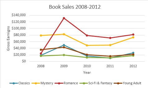The new chart type

To movement a chart:

Whenever you insert a new nautical chart, information technology will announced as an object on the same worksheet that contains its source data. Alternatively, you lot tin motion the nautical chart to a new worksheet to help keep your information organized.

Select the nautical chart yous want to move.
Click the Design tab, then select the Move Chart control.
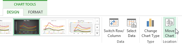Clicking the Move Chart command
The Motion Chart dialog box will appear. Select the desired location for the chart. In our case, we'll choose to motility it to a New sheet, which will create a new worksheet.
Click OK.
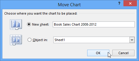Moving the chart to a new worksheet
The nautical chart will appear in the selected location. In our instance, the nautical chart at present appears on a new worksheet.
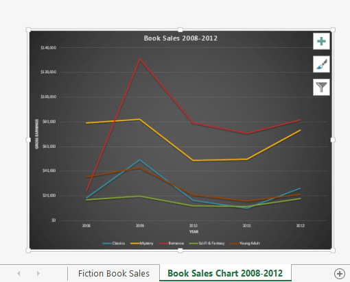The chart on its own worksheet

Keeping charts upwardly to date

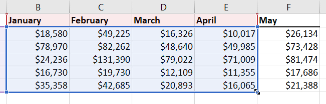
Past default, when yous add more than data to your spreadsheet, the chart may not include the new data. To fix this, you can arrange the data range. Just click the nautical chart, and it will highlight the data range in your spreadsheet. You can then click and drag the handle in the lower-right corner to modify the information range.

Screenshot of adjusting a data range

If you ofttimes add more data to your spreadsheet, it may get tiresome to update the data range. Luckily, there is an easier way. Simply format your source data as a table, so create a chart based on that table. When you add more data below the table, it volition automatically exist included in both the tabular array and the chart, keeping everything consistent and upwards to engagement.

Sentinel the video below to larn how to utilize tables to keep charts upwardly to date.

Challenge!

Open up an existing Excel workbook. If you want, you tin use our practice workbook.
Use worksheet data to create a nautical chart. If you are using the example, use the cell range A1:F6 as the source data for the chart.
Change the chart layout. If you are using the instance, select Layout viii.
Apply a nautical chart mode.
Motion the chart. If you lot are using the instance, movement the chart to a new worksheet named Volume Sales Data: 2008-2012.

/en/excel2013/sparklines/content/